VLSI lab
Remote Access to Linux Labs
- Connect to University VPN
- Open Remote Desktop Connection
- Computer: s2314951.studentlinux.eng.ed.ac.uk
- UserName: ED\s2314951
- In advanced -> Setting -> Use these RD gateway server setting:
- serverName: portico.is.ed.ac.uk
- Ok, connect
- quit the log in: System -> Log out
Normal Start Cadence
- Open Terminal
- Type ‘ssh vlx’
- Move into that directory - ‘cd AVLSIA’
- Type ‘avlsilaunch &’
Generate new cell
- Library Manager -> File -> New -> Library
- File -> New -> Cell View
Common parameters
New Instance: Create -> Instance -> Browse
| Instance | Library | Cell |
|---|---|---|
| NMOS | PRIMLIB | nmosm4 |
| PMOS | PRIMLIB | pmosm4 |
| Voltage source | analogLib | vdc |
| multi Voltage source | analogLib | vsource |
| Current source | analogLib | idc |
| Ground | analogLib | gnd |
| Resistor | analogLib | res |
| NAND | ahdlLib | nand_gate |
change parameters: click instance -> press Q
Draw line: Create -> Wire narrow
Note: remember click “check and save” after editing
ADE
- Launch -> ADE_L (open ADE)
- Analyses -> choose (choose analyses type)
- Output -> To be plotted -> choose node or branch in schemetic (plotted wave)
- Click run button on right bar (check again if schemetic is check and saved)
- Session -> Save state (save ADE)
- Session -> Load state
.tran
Based on time flowing, just select stop time
.dc
- Sweep Variable -> Component Parameter -> Select Component -> click wanted component in Schemetic
- fill Parameter type
- Sweep Range -> fill start value and stop value
- choose sweep type
.ac
- choose frequency analysis
- choose start and stop value
- choose logarithmic as sweep type
- fill 5 points per decade
Anaysis plot
Line: Marker -> Create marker -> Horizontal/Vertical
Press M to measure value on this point
And keep press D when first point is still selected, to measure distance and trend between two points
Press U to undo the operation
Calculator
- Tool -> Calculator
- Press “Wave” radio button to analysis wave values
- Press 7th icon on the bar under expression box to clear history memory
- Click Legend on plot window to input variable wave
- Choose functions on function panel
- Click Evaluate the buffer to plot the result (result will directly output in expression box if the result is a constant value)
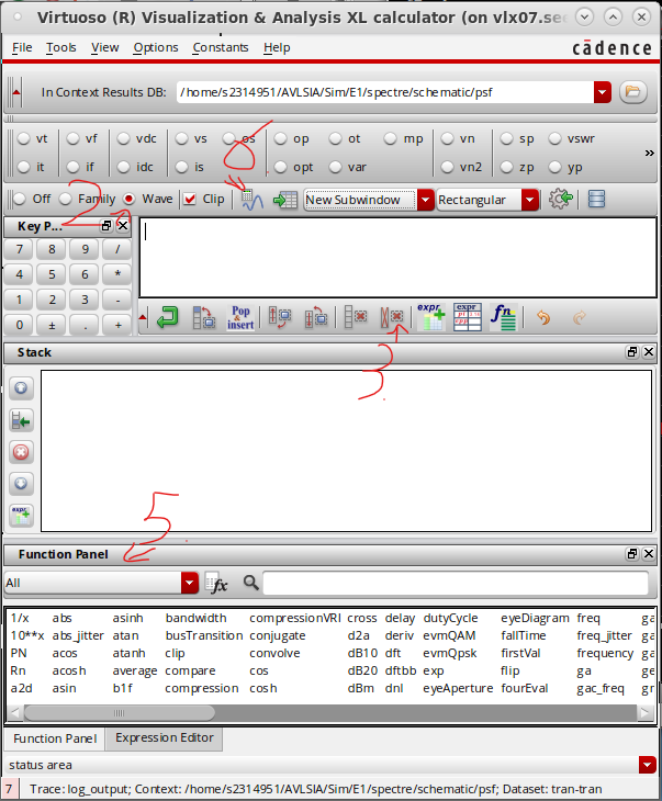
The calculated result can also be plotted automatically by placing expression in Output box in ADE_L:
Output -> Set up -> fill name -> phase expression, or press “Get Expression” (if there has an expression displayed in calculator already)
Parametic analysis
The second variable should be set up at first if you want change two variables in one simulation
- Let one parameter’s value into letter type (like Voltage=V)
- in ADE_L -> Variables -> Edit -> fill name and initialize value (like V=5)
- Tools -> Parametic analysis -> fill variable name, start and stop value -> select Step mode and step value or total point number
- Click green run button on top bar
ADE XL
Combining multiple simulation and schmetics in one window and control them together
Start a ADE_XL: open one schmatic -> launch -> ADE_XL -> Create New View -> XXX_ADE_XL (New XL cell will be generated)
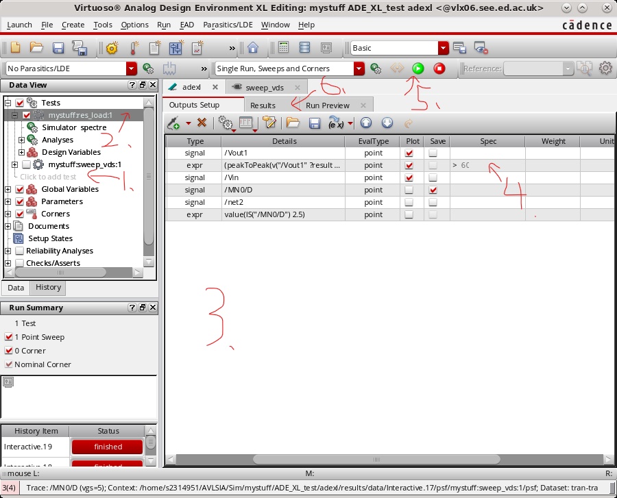
- click ‘Click to add test’ to select one schematic, and load state if have
- test editor is opened by double clicking here, Tests will automatically added from test editor
- expression can be added by right click region here, select ‘Add Expression’
- Only expressions and set specification here, by bouble clicking the grey area
- run the simulation. It can save up to 10 past histories
- Output results can be checked here
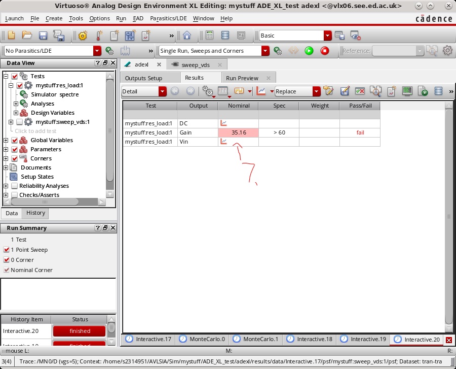
- wave polt can be displayed here
symbol
- in target cell, create -> Cell view -> From cellview -> OK
- set pins
- change the shape
- new cell view have generated in library menu
Mismatch simulation
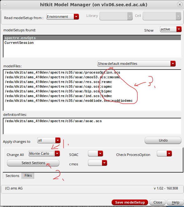
in virtuoso window, Hit-Kit Utilities -> Simulation Utilities -> Model Manager
- change the “change all” into ‘monte carlo’
- click ‘Select section’ making sure all parameters are end in ‘mc’ and click ‘Apply’ and ‘OK’
- double check all model files are end in ‘mc’ as well, and close window
now can open previous ADE_XL file
and check the sections are really chnaged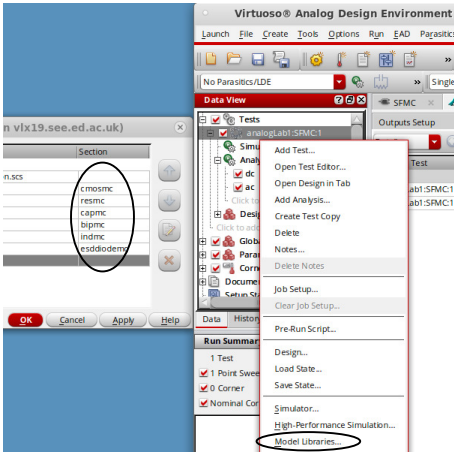
Now can add new expressions by right clicking blank area in working place, and ‘Add expression’
if we want measure the current when Voltage in drain terminal is 2.5V, can write as:
‘value(IS(“/MN0/D”) 2.5)’
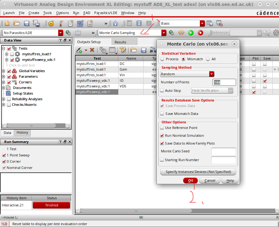
Now can go to monte carloanalysis.
- change the drop down menu into conte carlo type
- click OK after making sure everything is OK
- start the simulation
Set an Osillator by ring invertors

There have two global variables (svdd! and svss!) which also been set in invertor parameter.
Please note the initial condiction must be set on one wire, or the osillator will be happened
ADE_L -> simulation -> convergence aids -> initial condition -> set as 0 or 5V
and its better to choose 2.5V as a supply voltage, to drive it much similar as a real pulse signal
the little peaks which larger than supply voltage is porproated with CMOS area. less area CMOS has, lower peak the signal will have and will performed as a normal pulse signal
1Ring_Ocilattor1.png
and next can add a enable signal to control this pulse signal by NAND gate